Assembly Format

All assembly code in this post follows Intel syntax:

Operation Destination, Source

x86-64 General Purpose Registers

x86-64 architecture has 16 general purpose registers.

Special Registers

Among the 16 general purpose registers, %rbp and %rsp has special meanings that are not recommended to be changed by program.

%rsp is stack pointer, indicates the current address of the stack.

%rbp is base pointer, indicates the start address of a stack frame.

Hence, we should avoid using %rbp and %rsp when compiling a program.

Reserved Free Register

x86 supports a grammar like

ADD 8[%rsp], %r11d,

which is actually

MOV %r12d, 8[%rsp]
ADD %r12d, %r11d
MOV 8[%rsp], %r12d

Hence, we’d better reserve a free register for such usage.

By convention, this reserved register is %r11d.

And that makes available registers to 13.

Magic 13

Now you understand why x86-64 programs only have 13 general purpose registers to use.

Remember the magic number of 13 as we will begin discussing register allocation algorithms.

Division Registers

To perform division, x86 provides a very specific instruction called idivq S

The actual arithmetic happens here is:

%rax = (%rdx:%rax) / S
%rdx = (%rdx:%rax) % S

%rax stores quotient

%rdx stores remainder

: means concatenate %rdx and %rax together, with %rdx in the higher 64 bits and %rax in the lower 64bits.

This does not mean that we cannot allocate value to %rax and %rdx, but need to be extra careful when doing so.

Run Out of Registers?

Spilling is what will happen if a program runs out of registers. It means store a value on the stack.

As you must know, there is a huge gap in speed between accessing register and accessing main memory. Hence, if a program spills too much variables to stack, its performance will drop.

Hence, our program should allocate as less registers as possible onto stack.

Register Allocation Step by Step

Register Allocation is indeed an NP-Complete problem, so that we use a lot of approximation approaches here to solve it.

For example, determining if 2 temps interfere with each other is NP-Complete, so we used liveness and graph-based greedy algorithm to approximate it.

Step 0: What happens before register allocation?

The input of register allocation is an Abstract Assembly, preferably in Static Single Assignment (SSA) form.

SSA form means every var(temp) is assigned at most once, like

t0 <- 5 + 1
t1 <- t0 + 2
t2 <- 30
t3 <- t1 * t2

Step 1: Determine Liveness of Each Temp

Liveness basically means the time span of a temp’s existence in the code.

A temp t is live at line l if:

1. temp is read at line l
2. t is live at line l + 1 and not written at line l

For example:

t0 <- 5 + 1      # no temp is live at this line
t1 <- t0 + 2     # t0 is live because it is read, t1 is not live as it is written
t2 <- 30         # t1 is live because it is live at next line and not written
t3 <- t1 * t2    # t1 is live because it is read

A more real example:

main:
    x <− 42                  # None live
    t1 <− 2                  # x is live here
    t2 <− x % t1             # x and t1 are live here
    if (t2 == 0):            # t2 and x are liver here
        goto L1  
    else:
        goto L2
L1:
    x <− x + 1               # x is live here
    z <− 1                   # x is live here
    goto L3                  # z and x are live here
L2:
    t3 <− 1                  # x is live here
    z <− t3 * −1             # t3 and x are live here
    goto L3                  # z and x are live here
L3:
    %eax <− z * x            # z and x are live here
    return                   # eax live here beacuse it is read

Step 2: Build Interference Graph

The vertices of this graph are interference, which means that these 2 vertices existed in the same time and thus can not be allocated to the same register.

We have 2 ways to calculate interference:

Method 1

Add an edge between t1 and t2 if t1 and t2 are live at the same line.

Method 2

1. For d <- s1 + s2, add an edge between d and t, for every t live at next line.
2. For d <- s, add an edge between d and t for every t that t != s live at next line.

Usually, method 2 is better than method 1.

Step 3: Color the Graph

The next step is to color the interference graph. We will use number to represent colors. Since we only have 13 registers, we can only use 13 colors.

Greedy Coloring Algorithm

for c in 1 ... 13:
    for v in vertices:
        if v is not colored and v's neighbors are not colored in c:
            color v with c

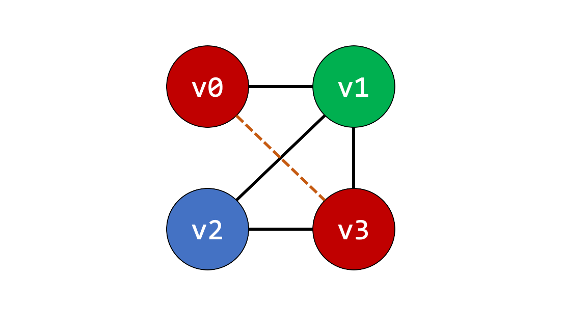
Not Perfect Answer

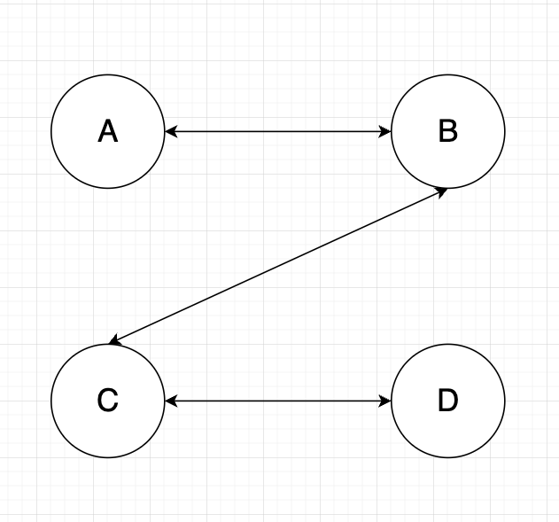
Different Ordering can produce different outcomes

A -> B -> C -> D: 2 colors

A -> D -> C -> B: 3 colors

Hence, we will run MSC algorithm to find optimal ordering before coloring the graph

Max Cardinality Search Algorithm

Input: An interference graph

Output: A ordering of vertices that will produce the minimum number of colors if used by greedy coloring

Algo

# set all weights to 0 initially
weight = {}
for v in vertices:
    weight[v] = 0

# find ordering
order = []
visited = set()
for i in range(number_of_nodes):
    v = node_with_max_weight
    order.append(v)
    for n in neighbor(v):
        if n not in visited:
            weight[n] += 1
    visited.add(v)

return order

Suppose we have the following interference graph:

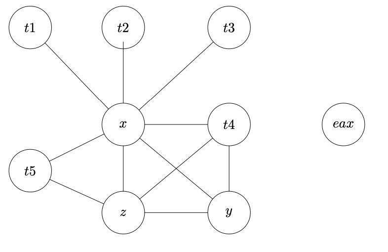
Suppose we pick t1 first, we will have ordering:

t1 -> x -> t2 -> t3 -> t5 -> z -> y -> t4 -> eax

Pre-Coloring

Some registers are reserved for special usage, and thus need special handling:

%rax is used to store return value. %rax and %rdx are used to store quotient and remainder in division.